Monitor system resources
Watch live CPU/memory/GPU graphs and apply synthetic load from the Monitor activity
Monitor system resources
The Monitor activity is HUB's htop-like live resource monitor: a scrolling stack of CPU heatmap, memory/swap, filesystem, disk/net I/O and GPU charts plus a process list. This guide covers the two things you drive from its toolbar — configuring the view and applying synthetic load for stability testing.
Open it
In HUB, open the Monitor activity from the menu. By default you see just a thin toolbar above the graphs — the monitor is for watching, so the controls stay out of the way until you summon them.
On Windows
The monitor reads the same things on Windows as on Linux, from the sources Windows' own tools use: CPU use per logical core with its user, kernel, DPC and interrupt shares; memory, the system cache and the paging file; each graphics adapter's load and video memory; disk and network rates; every fixed and removable drive; and every process with its CPU, memory, disk rates, GPU load and video memory.
Two things are not shown on Windows: CPU temperatures (Windows offers none without a vendor driver), and a process's command line (its image path is shown instead).
Configuring the view
Click the cog button in the toolbar to reveal the configuration panel; the graphs slide down to make room, and click again to hide it (the graphs reclaim the space). The open/closed state is remembered per node.
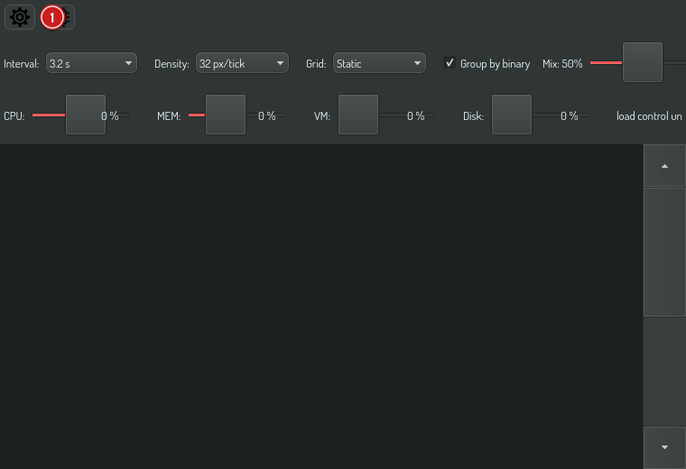
The panel holds five view controls:
- Interval — how often the monitor asks for a sample (50 ms – 5 s). It sets the cadence of the request, not a guarantee that a reading arrives; see When a graph shows red dots.
- Density — horizontal pixels per sample; lower values pack more history into the same width.
- Grid — Static keeps the time rulers fixed to the window (data scrolls under them); Follow data makes them wall-clock rulers that scroll with the data.
- Mix — blends every chart's color toward the shared base color.
- Group by binary — one row per program instead of one per process. See Reading the process list.
Reading the process list
Below the graphs, the process list shows what is using the machine, sorted by a blended usage score. Each row carries a heat strip of its own history.
When one program takes the whole list
A parallel linker or a compile farm forks dozens of times. Those processes have the highest scores on the machine, so they take the top dozens of rows, and your editor and your browser are pushed off the bottom. The list stops describing the machine at the moment you look at it.
Tick Group by binary in the configuration panel. The list folds to one row
per program: clang once instead of sixty-four times, with the resources of
all sixty-four added up.
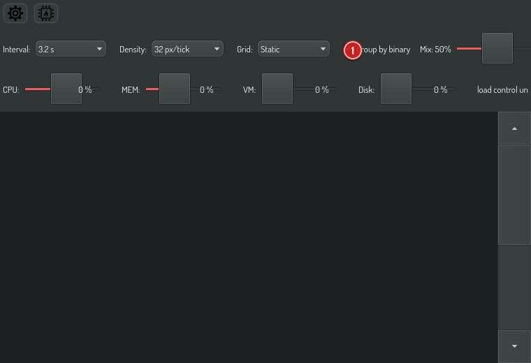
Nothing is hidden. A program running as a single process becomes a group of one, so every process is still on screen somewhere. The setting is remembered per node.
What a grouped row shows
- The PROCS column replaces the PID with the number of processes,
×64. - The COMMAND column shows the arguments those processes have in common.
When they do not all agree, it says so:
… 40 of 64means forty of the sixty-four share what you see, and the rest were invoked differently. - Hover a row for the shared path, the totals, and the five busiest members with their own pids — that is how you find which of the sixty-four is doing the work.
- Right-click for the group: copy every pid, the binary path, the shared command, or all of the command lines.
Two numbers worth understanding
Percentages are per core. 100% means one core's worth, for processor time
and for memory. A row reading 900 is using nine cores, or nine cores' worth
of memory. That keeps the two columns comparable at a glance.
Grouped memory is a sum and it over-counts. Processes of the same program share parts of their memory, and adding their figures counts those shared parts once for each process. Read a grouped memory figure as an upper bound. The hover tip says so too.
When a graph shows red dots
A small red dot under a graph column means the monitor took no measurement for that moment. An amber dot means it measured the levels — memory, swap, filesystem — but could not work out the rates for that column, because the reading arrived too late to divide by the time it covers.
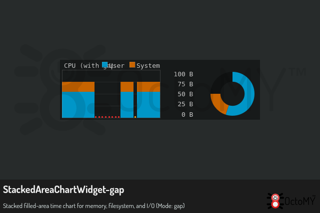
Where a dot appears, the graph leaves the column empty. That is deliberate. The monitor will not repeat the previous value or draw a zero, because both of those look exactly like a healthy idle machine — which is the opposite of what is happening. The process list dims for the same reason: the rows are still the last good reading, so they stay on screen rather than vanishing, but they are no longer current.
A run of red dots under heavy load is the monitor working correctly. Reading
the kernel's counters (/proc on Linux, the performance counters on Windows)
means waiting on the kernel, and a heavily loaded machine can make that
wait take seconds. The monitor keeps drawing on time and marks what it missed.
If dots appear on an idle machine, that is worth investigating — it points at storage or memory pressure rather than at the monitor.
Applying synthetic load
Click the stress button in the toolbar to open the synthetic-loads panel.
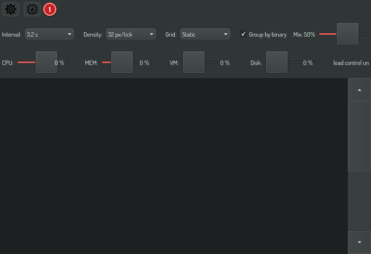
Drag the CPU load or MEM load slider and watch the effect live in the graphs above: the CPU heatmap reddens as cores saturate, and the memory chart's used band grows. There is no separate "on" switch — any non-zero percent is active, shown by the ● active chip; the danger-red Clear button drops all load in one click.
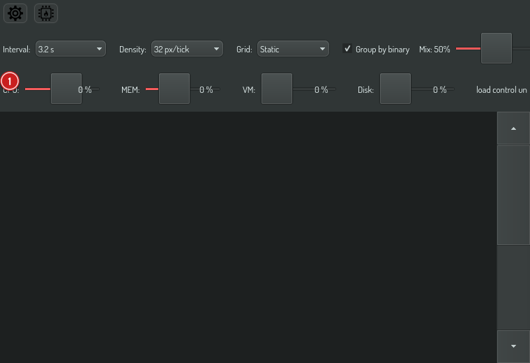
The load runs in a per-node service independent of this activity — it keeps running if you navigate away, and it is never persisted, so a fresh HUB always starts idle (a machine must never boot into self-inflicted load).
You can't lose the off switch
While any load is active, two safety affordances kick in:
- The loads panel cannot be hidden — the stress toggle locks open (its tooltip explains why). Press Clear first to unlock it.
- A danger-red return button appears in the header on every other screen. Click it to jump straight back to Monitor and the running sliders. It disappears the moment load drops to zero.
Together these guarantee the load controls are always one click away while the machine is under deliberate stress.
Applying load headlessly (OPAL)
For automated load-testing there is a system.load.* task family that drives
the very same service — so a load set this way shows up live in the graphs and
raises the same header return button:
hub --opal 'system.load.set cpu=50'
hub --opal 'system.load.status'
hub --opal 'system.load.clear'
See the system.load.* task reference for
the full parameter and output details.